For anyone unfamiliar with TensorTonic, it is often described as the “LeetCode of machine learning”, a platform designed for developers to practice algorithms, refine data science techniques, and build machine learning skills through hands-on coding challenges.

The problem statement

The Mean, Median, Mode problem on TensorTonic asks you to compute these three statistical metrics for a 1D numeric array. The updated requirements specify returning the results as a dictionary. If multiple values share the highest frequency, the mode must be the smallest of those values.

The time limit is 300ms, and you are permitted to use NumPy and the standard collections library.

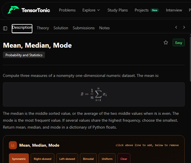
Here is the problem description as given on TensorTonic:

Compute three measures of a nonempty one-dimensional numeric dataset. The mean is:

$$\bar{x} = \frac{1}{n} \sum_{i=1}^{n} x_i$$

The median is the middle sorted value, or the average of the two middle values when $n$ is even. The mode is the most frequent value. If several values share the highest frequency, choose the smallest. Return mean, median, and mode in a dictionary of Python floats.

Examples

Input: x = [1, 2, 3, 4, 5]

Output: {“mean”: 3.0, “median”: 3.0, “mode”: 1.0}

Explanation: Every value appears once, so the smallest value wins the mode tie.

Input: x = [1, 2, 2, 3, 4]

Output: {“mean”: 2.4, “median”: 2.0, “mode”: 2.0}

Input: x = [1, 2, 3, 4]

Output: {“mean”: 2.5, “median”: 2.5, “mode”: 1.0}

Code samples

In case you just want the code, you can find them on my GitHub here.

The Standard Approach

Computing the mean and median is straightforward using NumPy. For the mode, the standard method tallies frequencies using collections.Counter, finds the highest frequency, filters all numbers sharing that frequency, and extracts the smallest one. The code below is from the solution on TensorTonic.

import numpy as np
from collections import Counter

def mean_median_mode(x):
    x = np.asarray(x, dtype=float)
    mean = float(np.mean(x))
    median = float(np.median(x))
    
    counts = Counter(x)
    max_count = max(counts.values())
    modes = [val for val, count in counts.items() if count == max_count]
    mode = float(min(modes))
    
    return {"mean": mean, "median": median, "mode": mode}

This functions correctly, but it traverses the unique values twice: first to find max_count, and again to build the modes list.

Single-Pass Optimization: Using max()

You can find the smallest mode in a single pass by providing a custom lambda function to Python’s built-in max() function.

import numpy as np
from collections import Counter

def mean_median_mode(x):
    x = np.asarray(x, dtype=float)
    mean = float(np.mean(x))
    median = float(np.median(x))
    
    counts = Counter(x)
    mode = float(max(counts, key=lambda k: (counts[k], -k)))
    
    return {"mean": mean, "median": median, "mode": mode}

When passing a tuple to Python’s max() function, it compares the first items. If they tie, it proceeds to the second items. The lambda lambda k: (counts[k], -k) maximizes the frequency count first. If counts tie, it maximizes the negative value of the key, which effectively selects the smallest original number.

Why this is better:

1. It’s faster ($O(N)$ instead of $2 \times O(N)$): Instead of traversing the unique values once for max() and a second time for the list comprehension, max() iterates through the keys exactly once.
2. It saves memory: It doesn’t need to create and store the intermediate modes list in memory.
3. It’s highly “Pythonic”: Using a tuple (primary_sort, secondary_sort) in a lambda function is the standard Python way to handle tie-breakers.

To understand why this lambda function is so clever, we have to look at how Python compares tuples.

When you give Python a tuple like (A, B), and ask it to find the maximum, it looks at the first item (A) first. If there is a tie, it looks at the second item (B) to break the tie.

Here is the exact breakdown of how lambda k: (counts[k], -k) uses that behavior to find the mode and handle ties in one swoop.

1. counts (What we are iterating over)

When you call max(counts, ...), Python iterates over the keys of the Counter dictionary. So k represents the actual numbers from your original array.

2. counts[k] (The Primary Sort: Find the most frequent)

The first part of the tuple is counts[k], which is the frequency of the number k.

Because max() wants the largest value, Python will first look for the key that has the highest count. If one number appears more than any other, it wins immediately, and Python ignores the second part of the tuple.

3. -k (The Secondary Sort: Break the tie)

If two numbers have the exact same frequency, Python moves to the second item in the tuple to break the tie.

We want to return the smallest number when there’s a tie, but max() is hardwired to look for the largest value.

By making the key negative (-k), we trick max() into doing what we want:

• Mathematically, -2 is greater than -5.
• So, if the numbers 2 and 5 are tied, max() will see -2 as the “larger” tie-breaker, and it will declare 2 the winner.

Let’s walk through a concrete example

Imagine your array is x = [8, 8, 3, 3, 1]. Both 8 and 3 appear twice. We want the mode to be 3 (the smaller of the tied values).

Here is what the lambda function calculates behind the scenes for each key:

• For k = 1: Count is 1. Tuple is (1, -1)
• For k = 8: Count is 2. Tuple is (2, -8)
• For k = 3: Count is 2. Tuple is (2, -3)

Now, Python’s max() function compares those tuples:

1. It instantly eliminates 1 because its primary value (1) is smaller than the others (2).
2. It compares (2, -8) and (2, -3).
3. Since the 2s tie, it compares -8 and -3.
4. Because -3 is greater than -8, the tuple (2, -3) wins.

The original key that generated that winning tuple was 3. Therefore, max() returns 3.

It is a brilliant, highly efficient way to tell Python: “Give me the item with the highest frequency, but if they tie, give me the one with the smallest numeric value.”

Single-Pass Optimization: Using min() (Hint 3)

The TensorTonic problem provides a hint suggesting the use of min(). You can invert the logic of the previous optimization to use min() instead, which reads highly intuitively for this specific constraint.

import numpy as np
from collections import Counter

def mean_median_mode(x):
    x = np.asarray(x, dtype=float)
    mean = float(np.mean(x))
    median = float(np.median(x))
    
    count = Counter(x)
    mode = float(min(count, key=lambda k: (-count[k], k)))
    
    return {"mean": mean, "median": median, "mode": mode}

By passing lambda k: (-count[k], k) to min(), Python evaluates the sequence as follows:

1. -count[k]: The min() function looks for the smallest number. By negating the count, the highest frequency becomes the most negative number, ensuring it is picked first.
2. k: If there is a tie in frequencies (the negative counts match), min() looks at the original numeric value k and simply selects the smallest one.

This completely satisfies the tie-breaking condition without needing negative key trickery on the secondary sort, making it an optimal, one-line solution for the mode.

So what’s the point?

All three versions spit out the same mean, median, and mode and the output never changes. What’s being shown here is a smaller habit: noticing when you’re looping over the same data twice, and finding a way to collapse that into one pass.

The tuple trick that makes this possible, where Python checks the first value and only falls back to the second if there’s a tie, isn’t specific to finding a mode. It shows up anywhere you’re sorting or picking “by this, then by that”: ranking search results, or breaking a tie between two players. The mode calculation is just a small, contained place to notice it and practice it.

Extra information for the reader - Measures of central Tendency

The rest of this post is optional but helpful for those who want to learn more about the concepts used in the solution from a theory perspective.

Central tendency describes where the “center” of a dataset lies. The three most common measures are:

• Mean: The arithmetic average
• Median: The middle value when data is sorted
• Mode: The most frequently occurring value

Each measure has different properties and is appropriate in different situations.

---

The Mean (Arithmetic Average)

The mean is the sum of all values divided by the count:

$$\bar{x} = \frac{1}{n} \sum_{i=1}^{n} x_i = \frac{x_1 + x_2 + ... + x_n}{n}$$

Properties:

• Uses all data points
• Sensitive to outliers
• Minimizes sum of squared deviations
• Has nice mathematical properties (unbiased estimator of population mean)

---

Computing the Mean: Example

Data: [4, 8, 6, 5, 3, 9, 7]

Step 1: Sum the values

$$4 + 8 + 6 + 5 + 3 + 9 + 7 = 42$$

Step 2: Count the values

$$n = 7$$

Step 3: Divide

$$\bar{x} = \frac{42}{7} = 6$$

The mean is 6.

---

The Median

The median is the middle value when data is sorted in order:

For odd $n$: The median is the value at position $\frac{n+1}{2}$.

For even $n$: The median is the average of values at positions $\frac{n}{2}$ and $\frac{n}{2} + 1$.

Properties:

• Robust to outliers
• Minimizes sum of absolute deviations
• Good for skewed distributions
• 50th percentile

---

Computing the Median: Odd $n$

Data: [4, 8, 6, 5, 3, 9, 7]

Step 1: Sort the data

$$[3, 4, 5, 6, 7, 8, 9]$$

Step 2: Find the middle position

$$\text{position} = \frac{n+1}{2} = \frac{7+1}{2} = 4$$

Step 3: The median is the 4th value

$$\text{median} = 6$$

---

Computing the Median: Even $n$

Data: [4, 8, 6, 5, 3, 9]

Step 1: Sort the data

$$[3, 4, 5, 6, 8, 9]$$

Step 2: Find the two middle positions

$$\text{positions} = \frac{n}{2} \text{ and } \frac{n}{2} + 1 = 3 \text{ and } 4$$

Step 3: Average the 3rd and 4th values

$$\text{median} = \frac{5 + 6}{2} = 5.5$$

---

The Mode

The mode is the value that appears most frequently:

Properties:

• Can be used with categorical data
• May not exist (if all values are unique)
• May not be unique (multimodal distributions)
• Not affected by outliers

---

Computing the Mode: Example 1

Data: [4, 8, 6, 5, 3, 6, 7, 6, 9]

Count occurrences:

• 3 appears 1 time
• 4 appears 1 time
• 5 appears 1 time
• 6 appears 3 times
• 7 appears 1 time
• 8 appears 1 time
• 9 appears 1 time

Mode = 6 (appears most frequently)

---

Computing the Mode: No Mode

Data: [4, 8, 6, 5, 3, 9, 7]

Each value appears exactly once. There is no mode (or we say all values are modes).

---

Computing the Mode: Multiple Modes

Data: [4, 8, 6, 5, 3, 6, 8, 9]

Count occurrences:

• 6 appears 2 times
• 8 appears 2 times
• All others appear 1 time

Modes = 6 and 8 (bimodal distribution)

---

Comparison: Mean vs Median

Symmetric distributions:

• Mean $\approx$ Median
• Either measure works well

Right-skewed distributions (long right tail):

• Mean > Median
• Median is often preferred

Left-skewed distributions (long left tail):

• Mean < Median
• Median is often preferred

With outliers:

• Mean is pulled toward outliers
• Median is robust to outliers

---

Effect of Outliers: Example

Data without outlier: [10, 12, 11, 13, 12, 11, 14]

$$\text{Mean} = \frac{10+12+11+13+12+11+14}{7} = \frac{83}{7} \approx 11.86$$

Median = 12 (middle of sorted [10, 11, 11, 12, 12, 13, 14])

Data with outlier: [10, 12, 11, 13, 12, 11, 100]

$$\text{Mean} = \frac{10+12+11+13+12+11+100}{7} = \frac{169}{7} \approx 24.14$$

Median = 12 (middle of sorted [10, 11, 11, 12, 12, 13, 100])

The outlier dramatically affects the mean but not the median.

---

When to Use Each Measure

Use Mean when:

• Data is roughly symmetric
• No significant outliers
• You need to use the value in further calculations
• You want to account for all values

Use Median when:

• Data is skewed
• Outliers are present
• Reporting “typical” values (e.g., income, house prices)
• Working with ordinal data

Use Mode when:

• Data is categorical
• You want the most common value
• Describing distribution shape (number of peaks)

Further Study

More detail can be found in the markdown file here, where we cover:

• Relationship in Different Distributions
• Weighted Mean
• Trimmed Mean
• Geometric Mean
• Harmonic Mean
• Relationship Between Means
• Central Tendency in Machine Learning
• Population vs Sample Notation
• Computational Considerations

Related Concepts & Posts

The following cards provide further definitions of concepts discussed above, and possible links to related posts.

TensorTonic Problem

Problem TensorTonic

TensorTonic is widely described as the LeetCode of machine learning, allowing developers to practice algorithms and build ML skills through interactive challenges.

Solve Challenge

NumPy Statistics Docs

Documentation NumPy

Official NumPy reference for statistical functions like mean and median.

View NumPy Docs

Python Counter Docs

Documentation Python

Python standard library documentation for collections.Counter.

View Python Docs